5. Inventory Dynamics#

GPU

This lecture was built using a machine with JAX installed and access to a GPU.

To run this lecture on Google Colab, click on the “play” icon top right, select Colab, and set the runtime environment to include a GPU.

To run this lecture on your own machine, you need to install Google JAX.

5.1. Overview#

This lecture explores the inventory dynamics of a firm using so-called s-S inventory control.

Loosely speaking, this means that the firm

waits until inventory falls below some value $s$
and then restocks with a bulk order of $S$ units (or, in some models, restocks up to level $S$ ).

We will be interested in the distribution of the associated Markov process, which can be thought of as cross-sectional distributions of inventory levels across a large number of firms, all of which

evolve independently and
have the same dynamics.

Note that we also studied this model in a separate lecture, using Numba.

Here we study the same problem using JAX.

We will use the following imports:

import matplotlib.pyplot as plt
import numpy as np
import jax
import jax.numpy as jnp
from jax import random, lax
from collections import namedtuple

Here’s a description of our GPU:

!nvidia-smi

Mon May 19 03:36:09 2025       
+-----------------------------------------------------------------------------------------+
| NVIDIA-SMI 575.51.03              Driver Version: 575.51.03      CUDA Version: 12.9     |
|-----------------------------------------+------------------------+----------------------+
| GPU  Name                 Persistence-M | Bus-Id          Disp.A | Volatile Uncorr. ECC |
| Fan  Temp   Perf          Pwr:Usage/Cap |           Memory-Usage | GPU-Util  Compute M. |
|                                         |                        |               MIG M. |
|=========================================+========================+======================|
|   0  Tesla T4                       Off |   00000000:00:1E.0 Off |                    0 |
| N/A   31C    P8             13W /   70W |       0MiB /  15360MiB |      0%      Default |
|                                         |                        |                  N/A |
+-----------------------------------------+------------------------+----------------------+
                                                                                         
+-----------------------------------------------------------------------------------------+
| Processes:                                                                              |
|  GPU   GI   CI              PID   Type   Process name                        GPU Memory |
|        ID   ID                                                               Usage      |
|=========================================================================================|
|  No running processes found                                                             |
+-----------------------------------------------------------------------------------------+

5.2. Sample paths#

Consider a firm with inventory $X_{t}$ .

The firm waits until $X_{t} \leq s$ and then restocks up to $S$ units.

It faces stochastic demand ${D_{t}}$ , which we assume is IID across time and firms.

With notation $a^{+} := max {a, 0}$ , inventory dynamics can be written as

\begin{array}{r} X_{t + 1} = {\begin{cases} (S - D_{t + 1})^{+} & if X_{t} \leq s \\ (X_{t} - D_{t + 1})^{+} & if X_{t} > s \end{cases} \end{array}

In what follows, we will assume that each $D_{t}$ is lognormal, so that

D_{t} = \exp (μ + σ Z_{t})

where $μ$ and $σ$ are parameters and ${Z_{t}}$ is IID and standard normal.

Here’s a namedtuple that stores parameters.

Parameters = namedtuple('Parameters', ['s', 'S', 'μ', 'σ'])

# Create a default instance
params = Parameters(s=10, S=100, μ=1.0, σ=0.5)

5.3. Cross-sectional distributions#

Now let’s look at the marginal distribution $ψ_{T}$ of $X_{T}$ for some fixed $T$ .

The probability distribution $ψ_{T}$ is the time $T$ distribution of firm inventory levels implied by the model.

We will approximate this distribution by

fixing $n$ to be some large number, indicating the number of firms in the simulation,
fixing $T$ , the time period we are interested in,
generating $n$ independent draws from some fixed distribution $ψ_{0}$ that gives the initial cross-section of inventories for the $n$ firms, and
shifting this distribution forward in time $T$ periods, updating each firm $T$ times via the dynamics described above (independent of other firms).

We will then visualize $ψ_{T}$ by histogramming the cross-section.

We will use the following code to update the cross-section of firms by one period.

@jax.jit
def update_cross_section(params, X_vec, D):
    """
    Update by one period a cross-section of firms with inventory levels given by
    X_vec, given the vector of demand shocks in D.

       * D[i] is the demand shock for firm i with current inventory X_vec[i]

    """
    # Unpack
    s, S = params.s, params.S
    # Restock if the inventory is below the threshold
    X_new = jnp.where(X_vec <= s, 
                      jnp.maximum(S - D, 0), jnp.maximum(X_vec - D, 0))
    return X_new

5.3.1. For loop version#

Now we provide code to compute the cross-sectional distribution $ψ_{T}$ given some initial distribution $ψ_{0}$ and a positive integer $T$ .

In this code we use an ordinary Python for loop to step forward through time

While Python loops are slow, this approach is reasonable here because efficiency of outer loops has far less influence on runtime than efficiency of inner loops.

(Below we will squeeze out more speed by compiling the outer loop as well as the update rule.)

In the code below, the initial distribution $ψ_{0}$ takes all firms to have initial inventory x_init.

def compute_cross_section(params, x_init, T, key, num_firms=50_000):
    # Set up initial distribution
    X_vec = jnp.full((num_firms, ), x_init)
    # Loop
    for i in range(T):
        Z = random.normal(key, shape=(num_firms, ))
        D = jnp.exp(params.μ + params.σ * Z)

        X_vec = update_cross_section(params, X_vec, D)
        _, key = random.split(key)

    return X_vec

We’ll use the following specification

x_init = 50
T = 500
# Initialize random number generator
key = random.PRNGKey(10)

Let’s look at the timing.

%time X_vec = compute_cross_section(params, \
        x_init, T, key).block_until_ready()

CPU times: user 1.41 s, sys: 211 ms, total: 1.62 s
Wall time: 1.2 s

Let’s run again to eliminate compile time.

%time X_vec = compute_cross_section(params, \
        x_init, T, key).block_until_ready()

CPU times: user 657 ms, sys: 159 ms, total: 816 ms
Wall time: 376 ms

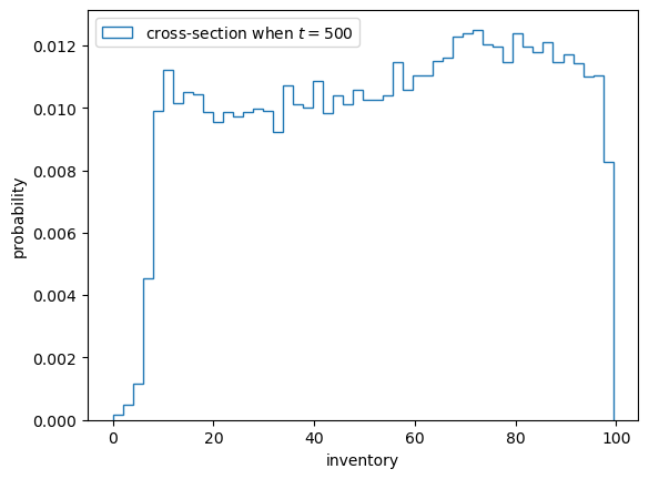
Here’s a histogram of inventory levels at time $T$ .

fig, ax = plt.subplots()
ax.hist(X_vec, bins=50, 
        density=True, 
        histtype='step', 
        label=f'cross-section when $t = {T}$')
ax.set_xlabel('inventory')
ax.set_ylabel('probability')
ax.legend()
plt.show()

_images/c6c1cf96342569dcccf3f7d888528ff87bef544c5d9356dfafe0add59e14cf09.png

5.3.2. Compiling the outer loop#

Now let’s see if we can gain some speed by compiling the outer loop, which steps through the time dimension.

We will do this using jax.jit and a fori_loop, which is a compiler-ready version of a for loop provided by JAX.

def compute_cross_section_fori(params, x_init, T, key, num_firms=50_000):

    s, S, μ, σ = params.s, params.S, params.μ, params.σ
    X = jnp.full((num_firms, ), x_init)

    # Define the function for each update
    def fori_update(t, inputs):
        # Unpack
        X, key = inputs
        # Draw shocks using key
        Z = random.normal(key, shape=(num_firms,))
        D = jnp.exp(μ + σ * Z)
        # Update X
        X = jnp.where(X <= s,
                  jnp.maximum(S - D, 0),
                  jnp.maximum(X - D, 0))
        # Refresh the key
        key, subkey = random.split(key)
        return X, subkey

    # Loop t from 0 to T, applying fori_update each time.
    # The initial condition for fori_update is (X, key).
    X, key = lax.fori_loop(0, T, fori_update, (X, key))

    return X

# Compile taking T and num_firms as static (changes trigger recompile)
compute_cross_section_fori = jax.jit(
    compute_cross_section_fori, static_argnums=(2, 4))

Let’s see how fast this runs with compile time.

%time X_vec = compute_cross_section_fori(params, \
                x_init, T, key).block_until_ready()

CPU times: user 610 ms, sys: 28.5 ms, total: 639 ms
Wall time: 517 ms

And let’s see how fast it runs without compile time.

%time X_vec = compute_cross_section_fori(params, \
                x_init, T, key).block_until_ready()

CPU times: user 7.86 ms, sys: 24 μs, total: 7.88 ms
Wall time: 9.56 ms

Compared to the original version with a pure Python outer loop, we have produced a nontrivial speed gain.

This is due to the fact that we have compiled the whole operation.

5.3.3. Further vectorization#

For relatively small problems, we can make this code run even faster by generating all random variables at once.

This improves efficiency because we are taking more operations out of the loop.

def compute_cross_section_fori(params, x_init, T, key, num_firms=50_000):

    s, S, μ, σ = params.s, params.S, params.μ, params.σ
    X = jnp.full((num_firms, ), x_init)
    Z = random.normal(key, shape=(T, num_firms))
    D = jnp.exp(μ + σ * Z)

    def update_cross_section(i, X):
        X = jnp.where(X <= s,
                  jnp.maximum(S - D[i, :], 0),
                  jnp.maximum(X - D[i, :], 0))
        return X

    X = lax.fori_loop(0, T, update_cross_section, X)

    return X

# Compile taking T and num_firms as static (changes trigger recompile)
compute_cross_section_fori = jax.jit(
    compute_cross_section_fori, static_argnums=(2, 4))

Let’s test it with compile time included.

%time X_vec = compute_cross_section_fori(params, \
                x_init, T, key).block_until_ready()

CPU times: user 420 ms, sys: 10.8 ms, total: 431 ms
Wall time: 379 ms

Let’s run again to eliminate compile time.

%time X_vec = compute_cross_section_fori(params, \
                x_init, T, key).block_until_ready()

CPU times: user 5.01 ms, sys: 0 ns, total: 5.01 ms
Wall time: 6.06 ms

On one hand, this version is faster than the previous one, where random variables were generated inside the loop.

On the other hand, this implementation consumes far more memory, as we need to store large arrays of random draws.

The high memory consumption becomes problematic for large problems.

5.4. Distribution dynamics#

Next let’s take a look at how the distribution sequence evolves over time.

We will go back to using ordinary Python for loops.

Here is code that repeatedly shifts the cross-section forward while recording the cross-section at the dates in sample_dates.

def shift_forward_and_sample(x_init, params, sample_dates,
                        key, num_firms=50_000, sim_length=750):

    X = res = jnp.full((num_firms, ), x_init)

    # Use for loop to update X and collect samples
    for i in range(sim_length):
        Z = random.normal(key, shape=(num_firms, ))
        D = jnp.exp(params.μ + params.σ * Z)

        X = update_cross_section(params, X, D)
        _, key = random.split(key)

        # draw a sample at the sample dates
        if (i+1 in sample_dates):
          res = jnp.vstack((res, X))

    return res[1:]

Let’s test it

x_init = 50
num_firms = 10_000
sample_dates = 10, 50, 250, 500, 750
key = random.PRNGKey(10)


%time X = shift_forward_and_sample(x_init, params, \
                    sample_dates, key).block_until_ready()

CPU times: user 1.28 s, sys: 284 ms, total: 1.57 s
Wall time: 991 ms

We run the code again to eliminate compile time.

%time X = shift_forward_and_sample(x_init, params, \
                    sample_dates, key).block_until_ready()

CPU times: user 1.03 s, sys: 239 ms, total: 1.27 s
Wall time: 603 ms

Let’s plot the output.

fig, ax = plt.subplots()

for i, date in enumerate(sample_dates):
    ax.hist(X[i, :], bins=50, 
            density=True, 
            histtype='step',
            label=f'cross-section when $t = {date}$')

ax.set_xlabel('inventory')
ax.set_ylabel('probability')
ax.legend()
plt.show()

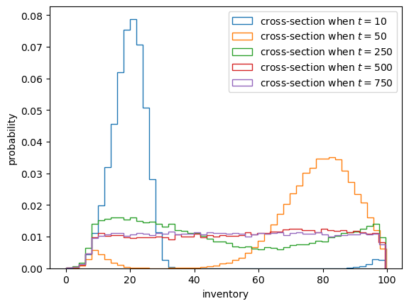
_images/597932d62260cb9c71dff44dbdfb3654aa77c958ba8319f7b55ec5b01a951a71.png

This model for inventory dynamics is asymptotically stationary, with a unique stationary distribution.

In particular, the sequence of marginal distributions ${ψ_{t}}$ converges to a unique limiting distribution that does not depend on initial conditions.

Although we will not prove this here, we can see it in the simulation above.

By $t = 500$ or $t = 750$ the distributions are barely changing.

If you test a few different initial conditions, you will see that they do not affect long-run outcomes.

5.5. Restock frequency#

As an exercise, let’s study the probability that firms need to restock over a given time period.

In the exercise, we will

set the starting stock level to $X_{0} = 70$ and
calculate the proportion of firms that need to order twice or more in the first 50 periods.

This proportion approximates the probability of the event when the sample size is large.

5.5.1. For loop version#

We start with an easier for loop implementation

# Define a jitted function for each update
@jax.jit
def update_stock(n_restock, X, params, D):
    n_restock = jnp.where(X <= params.s,
                          n_restock + 1,
                          n_restock)
    X = jnp.where(X <= params.s,
                  jnp.maximum(params.S - D, 0),
                  jnp.maximum(X - D, 0))
    return n_restock, X, key

def compute_freq(params, key,
                 x_init=70,
                 sim_length=50,
                 num_firms=1_000_000):

    # Prepare initial arrays
    X = jnp.full((num_firms, ), x_init)

    # Stack the restock counter on top of the inventory
    n_restock = jnp.zeros((num_firms, ))

    # Use a for loop to perform the calculations on all states
    for i in range(sim_length):
        Z = random.normal(key, shape=(num_firms, ))
        D = jnp.exp(params.μ + params.σ * Z)
        n_restock, X, key = update_stock(
            n_restock, X, params, D)
        key = random.fold_in(key, i)

    return jnp.mean(n_restock > 1, axis=0)

key = random.PRNGKey(27)

%time freq = compute_freq(params, key).block_until_ready()

CPU times: user 859 ms, sys: 60.3 ms, total: 919 ms
Wall time: 962 ms

We run the code again to get rid of compile time.

%time freq = compute_freq(params, key).block_until_ready()

CPU times: user 83.7 ms, sys: 17.4 ms, total: 101 ms
Wall time: 49.6 ms

print(f"Frequency of at least two stock outs = {freq}")

Frequency of at least two stock outs = 0.44772300124168396

Exercise 5.1

Write a fori_loop version of the last function. See if you can increase the speed while generating a similar answer.

Solution to Exercise 5.1

Here is a lax.fori_loop version that JIT compiles the whole function

@jax.jit
def compute_freq(params, key,
                 x_init=70,
                 sim_length=50,
                 num_firms=1_000_000):

    s, S, μ, σ = params.s, params.S, params.μ, params.σ
    # Prepare initial arrays
    X = jnp.full((num_firms, ), x_init)
    Z = random.normal(key, shape=(sim_length, num_firms))
    D = jnp.exp(μ + σ * Z)

    # Stack the restock counter on top of the inventory
    restock_count = jnp.zeros((num_firms, ))
    Xs = (X, restock_count)

    # Define the function for each update
    def update_cross_section(i, Xs):
        # Separate the inventory and restock counter
        x, restock_count = Xs[0], Xs[1]
        restock_count = jnp.where(x <= s,
                                restock_count + 1,
                                restock_count)
        x = jnp.where(x <= s,
                      jnp.maximum(S - D[i], 0),
                      jnp.maximum(x - D[i], 0))

        Xs = (x, restock_count)
        return Xs

    # Use lax.fori_loop to perform the calculations on all states
    X_final = lax.fori_loop(0, sim_length, update_cross_section, Xs)

    return jnp.mean(X_final[1] > 1)

Note the time the routine takes to run, as well as the output

%time freq = compute_freq(params, key).block_until_ready()

CPU times: user 511 ms, sys: 21.5 ms, total: 533 ms
Wall time: 468 ms

We run the code again to eliminate the compile time.

%time freq = compute_freq(params, key).block_until_ready()

CPU times: user 1.78 ms, sys: 146 μs, total: 1.93 ms
Wall time: 8.12 ms

print(f"Frequency of at least two stock outs = {freq}")

Frequency of at least two stock outs = 0.4476909935474396