10. Job Search#

GPU

This lecture was built using a machine with JAX installed and access to a GPU.

To run this lecture on Google Colab, click on the “play” icon top right, select Colab, and set the runtime environment to include a GPU.

To run this lecture on your own machine, you need to install Google JAX.

In this lecture we study a basic infinite-horizon job search problem with Markov wage draws

Note

For background on infinite horizon job search see, e.g., DP1.

The exercise at the end asks you to add risk-sensitive preferences and see how the main results change.

In addition to what’s in Anaconda, this lecture will need the following libraries:

!pip install quantecon

We use the following imports.

import matplotlib.pyplot as plt
import quantecon as qe
import jax
import jax.numpy as jnp
from collections import namedtuple

jax.config.update("jax_enable_x64", True)

10.1. Model#

We study an elementary model where

jobs are permanent
unemployed workers receive current compensation $c$
the horizon is infinite
an unemployment agent discounts the future via discount factor $β \in (0, 1)$

10.1.1. Set up#

At the start of each period, an unemployed worker receives wage offer $W_{t}$ .

To build a wage offer process we consider the dynamics

W_{t + 1} = ρ W_{t} + ν Z_{t + 1}

where $(Z_{t})_{t \geq 0}$ is IID and standard normal.

We then discretize this wage process using Tauchen’s method to produce a stochastic matrix $P$ .

Successive wage offers are drawn from $P$ .

10.1.2. Rewards#

Since jobs are permanent, the return to accepting wage offer $w$ today is

w + β w + β^{2} w + \dots = \frac{w}{1 - β}

The Bellman equation is

v (w) = max {\frac{w}{1 - β}, c + β \sum_{w^{'}} v (w^{'}) P (w, w^{'})}

We solve this model using value function iteration.

10.2. Code#

Let’s set up a namedtuple to store information needed to solve the model.

Model = namedtuple('Model', ('n', 'w_vals', 'P', 'β', 'c'))

The function below holds default values and populates the namedtuple.

def create_js_model(
        n=500,       # wage grid size
        ρ=0.9,       # wage persistence
        ν=0.2,       # wage volatility
        β=0.99,      # discount factor
        c=1.0,       # unemployment compensation
    ):
    "Creates an instance of the job search model with Markov wages."
    mc = qe.tauchen(n, ρ, ν)
    w_vals, P = jnp.exp(mc.state_values), jnp.array(mc.P)
    return Model(n, w_vals, P, β, c)

Let’s test it:

model = create_js_model(β=0.98)

model.c

1.0

model.β

0.98

model.w_vals.mean()  

Array(1.34861482, dtype=float64)

Here’s the Bellman operator.

@jax.jit
def T(v, model):
    """
    The Bellman operator Tv = max{e, c + β E v} with 

        e(w) = w / (1-β) and (Ev)(w) = E_w[ v(W')]

    """
    n, w_vals, P, β, c = model
    h = c + β * P @ v
    e = w_vals / (1 - β)

    return jnp.maximum(e, h)

The next function computes the optimal policy under the assumption that $v$ is the value function.

The policy takes the form

σ (w) = 1 {\frac{w}{1 - β} \geq c + β \sum_{w^{'}} v (w^{'}) P (w, w^{'})}

Here $1$ is an indicator function.

$σ (w) = 1$ means stop
$σ (w) = 0$ means continue.

@jax.jit
def get_greedy(v, model):
    "Get a v-greedy policy."
    n, w_vals, P, β, c = model
    e = w_vals / (1 - β)
    h = c + β * P @ v
    σ = jnp.where(e >= h, 1, 0)
    return σ

Here’s a routine for value function iteration.

def vfi(model, max_iter=10_000, tol=1e-4):
    "Solve the infinite-horizon Markov job search model by VFI."
    print("Starting VFI iteration.")
    v = jnp.zeros_like(model.w_vals)    # Initial guess
    i = 0
    error = tol + 1

    while error > tol and i < max_iter:
        new_v = T(v, model)
        error = jnp.max(jnp.abs(new_v - v))
        i += 1
        v = new_v

    v_star = v
    σ_star = get_greedy(v_star, model)
    return v_star, σ_star

10.3. Computing the solution#

Let’s set up and solve the model.

model = create_js_model()
n, w_vals, P, β, c = model

v_star, σ_star = vfi(model)

Starting VFI iteration.

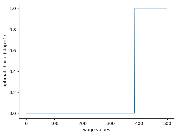
Here’s the optimal policy:

fig, ax = plt.subplots()
ax.plot(σ_star)
ax.set_xlabel("wage values")
ax.set_ylabel("optimal choice (stop=1)")
plt.show()

_images/37f92b538d37a0b6693cccc0cd2e7cd0db6a2f95f771c4b9c52d3216c2d2ec10.png

We compute the reservation wage as the first $w$ such that $σ (w) = 1$ .

stop_indices = jnp.where(σ_star == 1)
stop_indices

(Array([385, 386, 387, 388, 389, 390, 391, 392, 393, 394, 395, 396, 397,
        398, 399, 400, 401, 402, 403, 404, 405, 406, 407, 408, 409, 410,
        411, 412, 413, 414, 415, 416, 417, 418, 419, 420, 421, 422, 423,
        424, 425, 426, 427, 428, 429, 430, 431, 432, 433, 434, 435, 436,
        437, 438, 439, 440, 441, 442, 443, 444, 445, 446, 447, 448, 449,
        450, 451, 452, 453, 454, 455, 456, 457, 458, 459, 460, 461, 462,
        463, 464, 465, 466, 467, 468, 469, 470, 471, 472, 473, 474, 475,
        476, 477, 478, 479, 480, 481, 482, 483, 484, 485, 486, 487, 488,
        489, 490, 491, 492, 493, 494, 495, 496, 497, 498, 499],      dtype=int64),)

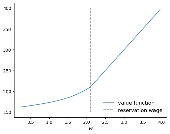
res_wage_index = min(stop_indices[0])

res_wage = w_vals[res_wage_index]

Here’s a joint plot of the value function and the reservation wage.

fig, ax = plt.subplots()
ax.plot(w_vals, v_star, alpha=0.8, label="value function")
ax.vlines((res_wage,), 150, 400, 'k', ls='--', label="reservation wage")
ax.legend(frameon=False, fontsize=12, loc="lower right")
ax.set_xlabel("$w$", fontsize=12)
plt.show()

_images/72b5dbe7759fc42dc33eb063f29db1473fd7b3a472279e651707faee1acb3239.png

10.4. Exercise#

Exercise 10.1

In the setting above, the agent is risk-neutral vis-a-vis future utility risk.

Now solve the same problem but this time assuming that the agent has risk-sensitive preferences, which are a type of nonlinear recursive preferences.

The Bellman equation becomes

v (w) = max {\frac{w}{1 - β}, c + \frac{β}{θ} \ln [\sum_{w^{'}} \exp (θ v (w^{'})) P (w, w^{'})]}

When $θ < 0$ the agent is risk averse.

Solve the model when $θ = - 0.1$ and compare your result to the risk neutral case.

Try to interpret your result.

You can start with the following code:

RiskModel = namedtuple('Model', ('n', 'w_vals', 'P', 'β', 'c', 'θ'))

def create_risk_sensitive_js_model(
        n=500,       # wage grid size
        ρ=0.9,       # wage persistence
        ν=0.2,       # wage volatility
        β=0.99,      # discount factor
        c=1.0,       # unemployment compensation
        θ=-0.1       # risk parameter
    ):
    "Creates an instance of the job search model with Markov wages."
    mc = qe.tauchen(n, ρ, ν)
    w_vals, P = jnp.exp(mc.state_values), mc.P
    P = jnp.array(P)
    return RiskModel(n, w_vals, P, β, c, θ)

Now you need to modify T and get_greedy and then run value function iteration again.

Solution to Exercise 10.1

RiskModel = namedtuple('Model', ('n', 'w_vals', 'P', 'β', 'c', 'θ'))

def create_risk_sensitive_js_model(
        n=500,       # wage grid size
        ρ=0.9,       # wage persistence
        ν=0.2,       # wage volatility
        β=0.99,      # discount factor
        c=1.0,       # unemployment compensation
        θ=-0.1       # risk parameter
    ):
    "Creates an instance of the job search model with Markov wages."
    mc = qe.tauchen(n, ρ, ν)
    w_vals, P = jnp.exp(mc.state_values), mc.P
    P = jnp.array(P)
    return RiskModel(n, w_vals, P, β, c, θ)


@jax.jit
def T_rs(v, model):
    """
    The Bellman operator Tv = max{e, c + β R v} with 

        e(w) = w / (1-β) and

        (Rv)(w) = (1/θ) ln{E_w[ exp(θ v(W'))]}

    """
    n, w_vals, P, β, c, θ = model
    h = c + (β / θ) * jnp.log(P @ (jnp.exp(θ * v)))
    e = w_vals / (1 - β)

    return jnp.maximum(e, h)


@jax.jit
def get_greedy_rs(v, model):
    " Get a v-greedy policy."
    n, w_vals, P, β, c, θ = model
    e = w_vals / (1 - β)
    h = c + (β / θ) * jnp.log(P @ (jnp.exp(θ * v)))
    σ = jnp.where(e >= h, 1, 0)
    return σ



def vfi(model, max_iter=10_000, tol=1e-4):
    "Solve the infinite-horizon Markov job search model by VFI."
    print("Starting VFI iteration.")
    v = jnp.zeros_like(model.w_vals)    # Initial guess
    i = 0
    error = tol + 1

    while error > tol and i < max_iter:
        new_v = T_rs(v, model)
        error = jnp.max(jnp.abs(new_v - v))
        i += 1
        v = new_v

    v_star = v
    σ_star = get_greedy_rs(v_star, model)
    return v_star, σ_star



model_rs = create_risk_sensitive_js_model()

n, w_vals, P, β, c, θ = model_rs

v_star_rs, σ_star_rs = vfi(model_rs)

Starting VFI iteration.

Let’s plot the results together with the original risk neutral case and see what we get.

stop_indices = jnp.where(σ_star_rs == 1)
res_wage_index = min(stop_indices[0])
res_wage_rs = w_vals[res_wage_index]

fig, ax = plt.subplots()
ax.plot(w_vals, v_star,  alpha=0.8, label="risk neutral $v$")
ax.plot(w_vals, v_star_rs, alpha=0.8, label="risk sensitive $v$")
ax.vlines((res_wage,), 100, 400,  ls='--', color='darkblue', 
          alpha=0.5, label=r"risk neutral $\bar w$")
ax.vlines((res_wage_rs,), 100, 400, ls='--', color='orange', 
          alpha=0.5, label=r"risk sensitive $\bar w$")
ax.legend(frameon=False, fontsize=12, loc="lower right")
ax.set_xlabel("$w$", fontsize=12)
plt.show()

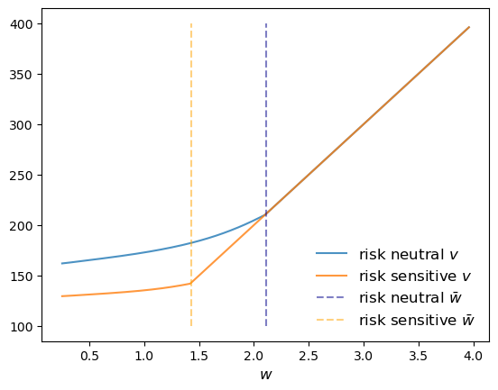
_images/e9783e98f9243d0eacfd26651a9967a32632a0196b5280c4c558de33b37e7622.png

The figure shows that the reservation wage under risk sensitive preferences (RS $\bar{w}$ ) shifts down.

This makes sense – the agent does not like risk and hence is more inclined to accept the current offer, even when it’s lower.